Flocking Per Second
As implied in the title, this post is all about flocking. This task was divided into three parts, the first of which being optimisation and will be the main focus herein. To set the scenario, my peers and I were provided with a 2D flocking simulation in C++. The simulation itself including the scene layout was hard coded, written in such a way that it was easy to understand but by no means fast. The end goal that is part B, was to eventually have the program be user configurable without having to edit any source code through some form of input. Following on from this is part C, having the program output useful information for the purpose of reviewing and tweaking the simulation further.
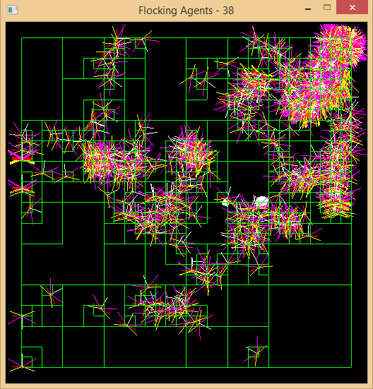
The first step in handling larger quantities of simulated agents at an acceptable rate, was the addition of multithreading using OpenMP. This was achieved by parallelising the core update loops for the scene, doubling the performance in most cases. The next stage of optimisation and by far the most significant was the introduction of spatial partitioning. Using the knowledge I obtained on Octrees from the ray tracing task, Quadtrees were the obvious choice for this 2D simulation. In the image above, the green lines represent the layout of the Quadtree at any given time.
Unlike use of a static Octree for the ray tracer, a dynamic structure capable of handling thousands of moving entities in real-time was required. As there were no memory limitations, the approach I chose was to construct every node of the Quadtree during scene initialisation, up to a specified depth. The key here was that each node contained an extra flag, indicating whether or not it was occupied either directly as a leaf node or further down the hierarchy. This allowed for entities to be removed or inserted on the fly, when used in conjunction gives the illusion that an entity has shifted regions.
The results from spatial partitioning varied excessively depending on how spread out agents are from each other, which in the case of flocking are often very close. Due to the sensor range when clumped together, performance can actually slightly worsen given the extra overhead of traversal. In a general case however, once agents begin to spread out the performance increase is exponential. The final stage of optimisation included basic rearrangements of mathematical operators, precomputation of commonly used values and the removal of header bloat for more efficient compilation times.
For parts B and C, I wrote a simple CSV reader that I later expanded upon with support for writing. This formed the basis for I/O, with separate CSV files for specifying agents, obstacles and simulation settings. As agents can be either prey or a predator, the ability for predators to kill prey was added and statistics logged during runtime. At the end of the simulation, a CSV file is written out containing the average, standard deviation and five number summary of predator kills. To compliment this information, two heatmaps displaying the position of agents as they move and where they were killed if applicable are also saved on exit.


Comments
Post a Comment